Kaiser Rule
Dozens of different methods have been developed for selecting the number of factors; the three most common are described below.
All the methods employed are Heuristics, which is to say none can be shown to be valid and each can make sense in some circumstances. For this reason, the general advice is to use these different rules as a starting point and then select a number of components such that the resulting components seem valid (see Validating Principal Components Analysis).
Kaiser Rule
The more variables that load onto a particular component (i.e., have a high correlation with the component), the more important the factor is in summarizing the data. An eigenvalue is an index that indicates how good a component is as a summary of the data. An eigenvalue of 1.0 means that the factor contains the same amount of information as a single variable. [note 1]
The Kaiser Rule is the most commonly used approach to selecting the number of components and it is the default in most programs.
It has been criticized on the grounds that it sometimes results in the selection of too many components.[1]
Scree plot
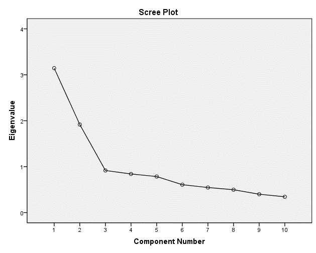
The following scree plot shows the number of Eigenvalues from the example shown on the main principal components analysis page, ordered from biggest to smallest. Some researchers conclude that the correct number of components is the number that appear prior to the elbow (in this example, two).
Proportion of variance explained
It is sometimes thought that a good factor analysis should explain two-thirds of the variance. Using the example presented in the main principal components analysis page, this leads to selection of a four component solution.
Notes
- ↑ Although this is the intuition behind the Kaiser Rule it is not a precisely accurate description because it ignores the capitalization upon chance that is guaranteed with principal components analysis.
References
- ↑ Nunnally, J. C. and I. H. Bernstein (1994). Psychometric Theory. New York, McGraw-Hill.
